Next-generation simulation

Is your simulation
too slow?
Ours isn't.

Discrete Rate Simulation — the paradigm that replaces event-by-event tracking with rate-based flow calculation. Any system with rates, constraints, and variability. Manufacturing. Healthcare. Logistics. Cutting-edge speed. Independently validated within 1%.

See the paradigm ↓ What can you model? ↓
Why it's fast

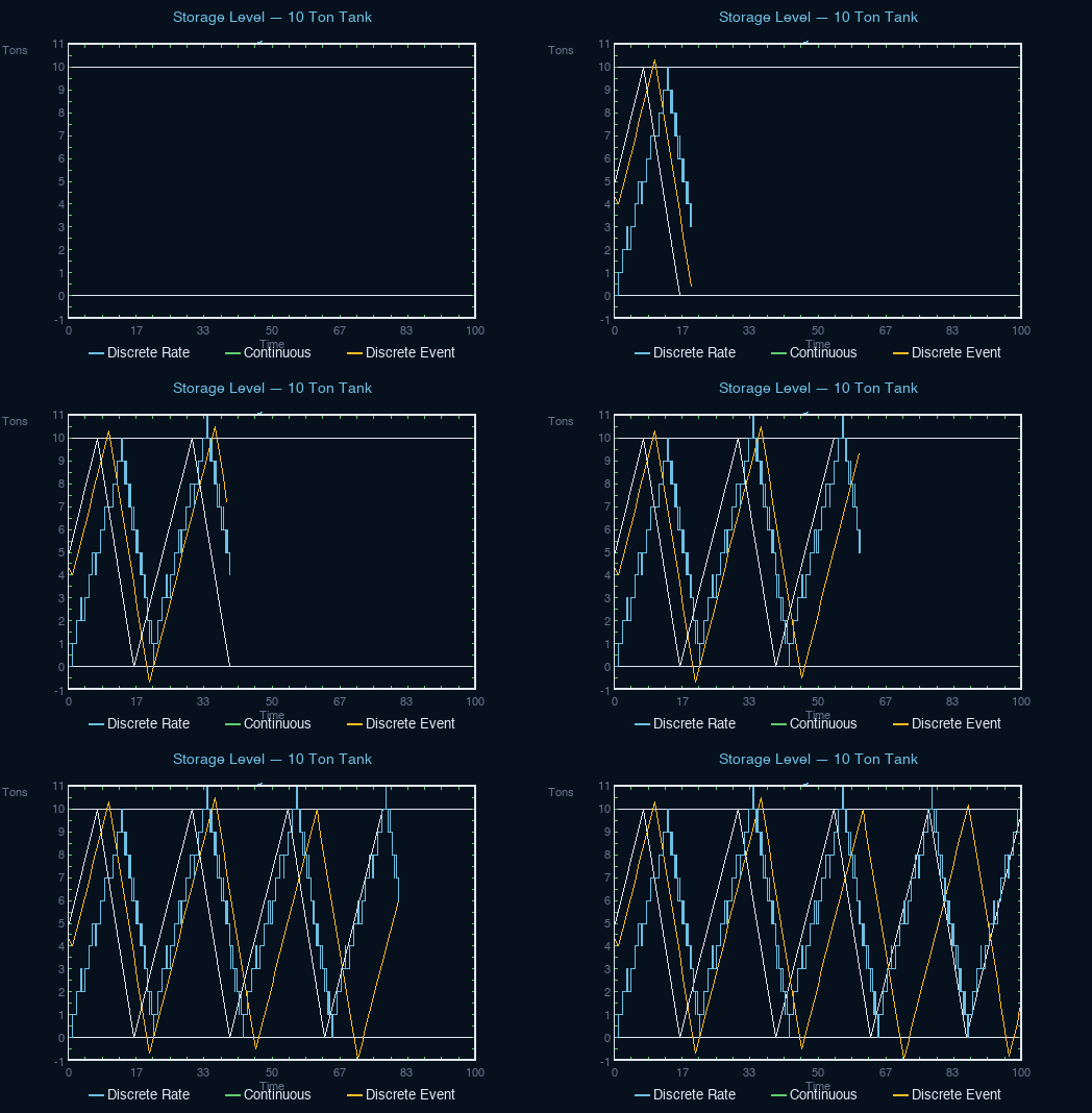
Same system. Three simulation approaches.

This simple example shows why Discrete Rate is so fast. Discrete Event tracks every individual item — thousands of events for a single tank fill. Continuous recalculates at every time slice whether anything changed or not. Discrete Rate only fires when something actually changes: 4 events total — start, full, empty, end. Between events, the rate is constant. No recalculation needed. Scale that to a real system and the difference is orders of magnitude.

Animated comparison of continuous, discrete rate, and discrete event simulation tracking a tank level
The building blocks

Three primitives.
Any rate-based system. Any industry.

Every discrete rate model is built from three fundamental block types — first introduced by Andrew Siprelle in 1992 and now used by tens of thousands of practitioners worldwide.

Constraint
Constraint

The Process

Anything that moves or transforms material at a defined rate — a treatment stage, reactor, filling station, processing unit, or service point. Rate is primary; individual entities are not tracked.

Rate-based Throughput Changeover
Buffer
Buffer

The Storage

Inventory, tanks, accumulators, or conveyors between operations. Buffers absorb rate mismatches and decouple upstream failures from downstream starvation.

Accumulator Inventory Decoupling
Interrupt

The Event

Anything that changes a rate — a failure, jam, scheduled break, or wear event. Three types govern how and when a constraint resets back to running.

Competing Cumulative wear Wall clock
Competing

Multiple failure modes compete to occur. After any stop, the clock resets — the next disruption starts fresh. Models random breakdowns, surges, and unplanned events.

Scheduled

Triggered by time — shift changes, maintenance windows, planned outages. Predictable, recurring, and independent of process state.

The problem

Where traditional simulation
loses the plot.

Discrete Event Simulation was built for a different era. Push it into a modern high-speed line and three things fail — fast.

Event explosion

A 1,000 unit/min line fires millions of events per simulated hour. Models slow to a crawl or become unrunnable at production scale.

Fidelity loss

Micro-stoppages, blocking, starvation, and cascading failures get rounded away. What remains is a clean model of a messy reality that doesn't exist.

Wrong paradigm

High-speed lines don't behave like queues. They behave like flow networks under disruption. Modeling them as events is the wrong abstraction from the start.

The solution

What is Discrete Rate Simulation?

Continuous Flow
+
Interrupting Events
=
System State

Flow is primary. Events modify it. State evolves continuously — never approximated, never rounded.

Upstream
Blocked
1,200 → 0/min
Buffer
Full
decoupler
Interrupt
STOP
8.4 min TTR
Downstream
Starved
cascade effect
Buffer full →
upstream blocked
Absorbs
rate mismatch
Event
modifies flow
Cascading Losses
Side by side

How they differ.

Discrete Event Simulation
Discrete Rate Simulation
Each unit is an individual event
Flow is modeled as a rate, not unit-by-unit
Performance degrades with line speed
Complexity is independent of throughput rate
Micro-stoppages averaged away
Every interrupt modeled explicitly with TTF/TTR distributions
Blocking & starvation approximated
Flow propagation captures blocking and starvation exactly
Models validate at low speeds, fail at scale
Independently validated within 1% of actual production at full scale

"It would take me up to a month to develop a digital twin for a production line using traditional methods. ChiAha's discrete rate approach streamlines this process while still delivering high-quality results."

— Tom Lange, Technology Optimization & Management LLC · 36 years, Procter & Gamble · Co-author, "High Accuracy Discrete Rate and Reliability Modeling" (WSC 2020) · Independently validated within 1% OEE accuracy

Where it works

Any system with rates, constraints, and variability.

If things flow through your system at a rate, and interruptions disrupt that flow — discrete rate is the right paradigm.

🧴

Bottling & Packaging

High-speed filling, capping, and labeling lines where a 3-second micro-stop cascades through four downstream stations.

💊

Pharma & Life Sciences

Regulated, tightly coupled processes where every interruption must be modeled precisely for compliance and capacity planning.

🏥

Hospital Patient Flow

ED arrivals, bed turnover, discharge rates, shift changes. The constraint shifts by hour — simulation reveals which interventions matter when.

⚗️

Chemical & Continuous Process

Reactors, distillation columns, heat exchangers. Progressive rate degradation from fouling is an interrupt — not just on/off failures.

🚰

Water & Wastewater

Treatment stages with scheduled backwash cycles, seasonal demand variation, and parallel unit constraint shifts.

Power Generation

Combined cycle plants with rated outputs, forced outages, and partial derating — the system doesn't stop, but the constraint tightens.

🥫

Food & Dairy Processing

Continuous flow with CIP cycles, quality windows, and cold chain constraints. Buffer sizing isn't just throughput — it's product integrity.

🔬

Semiconductor & Electronics

Batch and flow processes with ultra-low cycle times and yield events that ripple through entire fab lines.

🛢️

Oil & Gas Pipelines

Compressor stations, metering points, line pack as buffer. When a compressor trips, the pipeline is a constraint system.

🧪

Specialty Materials

Small-batch production with tight quality windows, long changeovers, and cure times. Rate shifts with composition; yield events behave like scheduled interrupts.

🚛

Fleets

Trucks, rail, or mobile equipment as a system. Vehicle availability is the constraint; maintenance cycles, refueling, and driver hours behave exactly like interrupts on a line.

The core mechanic

The Interrupt Construct.

Every disruption is modeled as an interrupt — with its own statistical distribution for time-to-failure and time-to-repair. No averaging. No aggregation. The full competing-risk picture.

Filler A
94.2%
Filler B ←
81.3%
Capper
97.1%

Two fillers. Same total downtime. Filler B's frequent short stops create compounding starvation — and recover 220+ more minutes when fixed. That's what the interrupt construct reveals.

The real value

Most tools show you
what happened.
This shows you
what will happen if you change it.

What if we increase line speed by 5%?
1,200
Current
1,188
+5% speed
↓ Net gain suppressed by Filler B starvation
What if we fix Filler B's interrupts first?
1,200
Current
1,347
Fix B first
↑ +12.3% effective throughput
What if we add a vision inspection station?
98.2%
Without
99.7%
With vision
↑ Quality yield at 1% speed reduction tradeoff
What if we change the buffer between stations 3 and 4?
14.2%
Starvation now
4.1%
+30 unit buffer
↓ 71% reduction in downstream starvation
Peer-reviewed

35 years of published research.

Discrete Rate Simulation has been validated, benchmarked, and extended across peer-reviewed publications since 1995 — from WSC to Springer to HMS proceedings.

View all publications → chiaha.com/research
The tools

Built on this paradigm.

The DiscreteRate paradigm powers ReliaSim — manufacturing-deep simulation validated within 1% OEE — plus a free web-based Decoupling Buffer Simulator anyone can try.

ReliaSim Available Now See ReliaSim →

Manufacturing-deep simulation with detailed failure modes, TTF/TTR distributions, blocking/starving analysis, and Gain ≠ Loss experimentation. Independently validated within 1% OEE.

Decoupling Buffer Simulator Free · Open Access Try it →

Web-based discrete rate simulation for decoupling buffer design. Explore production lines with buffers, breakdowns, and speed variance. No login — test any scenario in your browser.

94.2%
OEE Predicted
1,138
Units/min Actual
4.9
Stops/Shift
Filler A97.1%
Filler B81.3%
Capper94.2%
Labeler98.8%
SIMULATION RESULT
Fix Filler B → recover +220 min/shift vs. identical downtime on Filler A
Stay connected

Join our list

Product updates, case studies, and fresh insights — straight to your inbox. No spam.
